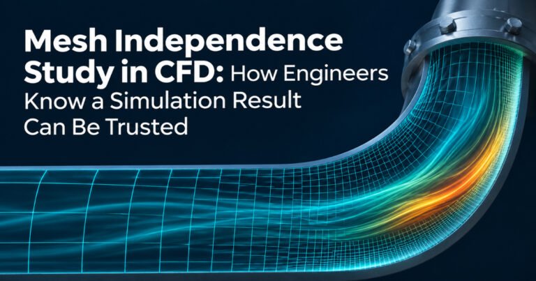
A practical guide to grid convergence, the Grid Convergence Index, and the mistakes that quietly undermine CFD results.
Every CFD solver will give you an answer. The residuals fall, the contours look smooth, and a colourful velocity plot is ready for the report. But a converged simulation is not necessarily an accurate one. If the mesh is too coarse, the result may say more about the grid than about the physics, and a design decision built on it can be wrong.
A mesh independence study, also called a grid convergence study, is the standard way to find out. It checks whether the quantities you care about, such as pressure drop, drag or peak temperature, stop changing meaningfully as the mesh is refined. This article covers why it matters, how to run one step by step, how to quantify the remaining error with the Grid Convergence Index (GCI), and the mistakes that quietly undermine otherwise careful work.
Why the Mesh Matters
Finite-volume CFD divides the flow domain into small cells and solves discretised versions of the conservation equations on each one. The difference between that discretised solution and the exact solution of the equations is the discretisation error, and it shrinks as the cells get smaller. Coarse meshes typically smear boundary layers through numerical diffusion, mis-predict flow separation and reattachment, and over- or under-estimate pressure losses and heat transfer.
Refinement is not free. In three dimensions, halving the cell size multiplies the cell count by eight, and transient simulations also need smaller time steps, so the cost can rise by an order of magnitude or more. The goal is therefore not the finest possible mesh. It is the coarsest mesh whose answers are acceptably close to what an infinitely fine mesh would give.
What a Mesh Independence Study Actually Checks
The study runs the same case on a series of systematically refined meshes and compares chosen output quantities. When the change between successive meshes becomes small, the solution is considered mesh independent. Strictly speaking, no result is ever perfectly independent of the mesh. What we really estimate is how large the remaining discretisation error is. That is why modern practice, following the ASME V&V 20 standard and the procedure published by Celik et al. (2008), reports an error band rather than a simple yes or no.
Step-by-Step: How to Run a Mesh Independence Study
Step 1: Choose your quantities of interest. Residuals tell you the solver has settled. They do not tell you the answer is right. Pick outputs tied to the engineering decision: pressure drop across a valve, drag coefficient of a vehicle, area-averaged outlet temperature of a heat exchanger, mass-flow split between branches, or maximum component temperature. Where relevant, also compare profiles, such as velocity along a line, because integral values can hide local errors.
Step 2: Build at least three meshes. Generate a coarse, medium and fine mesh with the same method, cell types and growth settings, so that resolution is the only thing that changes. A refinement ratio of at least 1.3 between successive meshes is recommended so the differences stand out from numerical noise. The ratio is defined using a representative cell size, h = (V/N)^(1/3) in 3D, where V is the domain volume and N is the number of cells.
Step 3: Keep everything else identical and converge every run. Use the same solver, discretisation schemes, turbulence model and boundary conditions. Converge each case properly: residuals dropped, monitored quantities flat, and global mass and energy balances closed. A poorly converged fine mesh can look worse than a well-converged coarse one and send you chasing the wrong problem.
Step 4: Compare the results. Tabulate each quantity of interest for every mesh and plot it against h. If the curve flattens as h decreases, you are approaching the mesh-independent value.
Step 5: Quantify the error with the GCI. Let f1, f2 and f3 be the results on the fine, medium and coarse meshes, and r the constant refinement ratio.
- Apparent order of convergence: p = ln[(f3 − f2) / (f2 − f1)] / ln(r)
- Richardson-extrapolated value: f_ext = f1 + (f1 − f2) / (r^p − 1)
- Fine-mesh GCI: GCI = 1.25 × |(f2 − f1) / f1| / (r^p − 1)
The factor 1.25 is the safety factor recommended when three or more meshes are used. The apparent order p should sit near the formal order of your numerical scheme, about 2 for second-order schemes. A value far from that is a warning that something is off.
Step 6: Select and document the mesh. Choose the coarsest mesh whose GCI is below the accuracy the decision requires, and record the meshes, settings and GCI in your project report.
A Worked Illustration
The numbers below are illustrative and chosen to show the calculation. They are not project data. Suppose we simulate the pressure drop through a manifold on three meshes with a constant refinement ratio of about 1.44:
- Coarse mesh (0.6 million cells): 1,201 Pa
- Medium mesh (1.8 million cells): 1,180 Pa
- Fine mesh (5.4 million cells): 1,170 Pa
The change from coarse to medium is about 1.8%, and from medium to fine about 0.85%. The apparent order works out to p ≈ 2.0, consistent with a second-order scheme. The extrapolated value is about 1,161 Pa and the fine-mesh GCI is about 1%. We can therefore report the pressure drop as roughly 1,170 Pa with a numerical uncertainty near 1%. The medium mesh would carry about 2% uncertainty. If the project can tolerate that, it delivers the answer with about two-thirds fewer cells.
Common Mistakes
- Judging by residuals instead of outputs. Low residuals show the equations are balanced, not that the answer is mesh-independent.
- Uneven or inconsistent refinement. Local refinement in high-gradient regions is legitimate, but it must be applied consistently across the whole series. Otherwise the cell-size metric used in the GCI calculation loses its meaning.
- Forgetting the wall. Wall functions assume the first cell sits in the log-law region (y+ roughly 30 to 300). Refining near the wall can push y+ into the buffer layer, where wall functions are unreliable, so the result can get worse as the mesh gets finer. Either keep y+ in the wall-function range on all meshes or resolve the viscous sublayer (y+ close to 1) on all of them.
- Ignoring cell quality. Skewness, orthogonal quality and aspect ratio matter. A fine mesh full of distorted cells can perform worse than a clean coarse one.
- Not refining the time step. In transient runs, refine the time step along with the mesh so the Courant number stays comparable.
- Ignoring non-monotonic behaviour. If the result rises and falls as the mesh is refined, the standard GCI formulas do not apply directly. Add meshes or look for the cause, which is often poor cell quality or unsteadiness.
Mesh Independence Is Not Validation, It Is Just Verification
A mesh-independent result tells you the equations are being solved accurately. It says nothing about whether those equations, with their turbulence model, boundary conditions and material properties, represent reality. That second question is validation, and it requires comparison with experimental data. We will cover it in our upcoming guide blogs.
Practical Tips for Industrial Projects
- Debug the set-up on a coarse mesh and refine only once the physics and boundary conditions are settled.
- Use symmetry and sector models to afford finer meshes where the geometry allows.
- Apply solution-adaptive refinement for features such as shocks, flames and free surfaces, as in our computational study of aerospike nozzles.
- Run the study at the most demanding operating point (highest Reynolds number or power) and reuse that resolution across a family of design variants. This also keeps simulation data consistent when building surrogate models for design optimisation.
How Experiqs Approaches It
At Experiqs, a mesh independence study is a standard step in every CFD project, whether it supports CFD-based flow path optimisation for industrial equipment, process flow optimisation in oil and gas or data center cooling performance. Our PhD-led teams combine industry-standard solvers with high-performance computing and, where needed, experimental validation, so results can stand up in a design review. Explore our Simulation & Validation services or start an R&D discussion with our engineers.
References
[1] I.B. Celik, U. Ghia, P.J. Roache, C.J. Freitas, H. Coleman and P.E. Raad, “Procedure for Estimation and Reporting of Uncertainty Due to Discretization in CFD Applications,” Journal of Fluids Engineering, vol. 130, no. 7, 078001, 2008.
[2] P.J. Roache, Verification and Validation in Computational Science and Engineering. Hermosa Publishers, 1998.
[3] ASME V&V 20-2009, Standard for Verification and Validation in Computational Fluid Dynamics and Heat Transfer. ASME, 2009.
[4] H.K. Versteeg and W. Malalasekera, An Introduction to Computational Fluid Dynamics: The Finite Volume Method, 2nd ed. Pearson, 2007.
[5] J.H. Ferziger and M. Perić, Computational Methods for Fluid Dynamics, 3rd ed. Springer, 2002.